What is a transient?

Why current and speed cannot change instantly, and how to read time responses.

Why study the motion between operating points?

Pressing a start button takes an instant; a motor takes time to accelerate. During this interval, current, electromagnetic torque and speed differ from their steady-state values. Peak currents, speed dips and mechanical stresses often occur here. A rated power alone cannot describe starting behaviour.

A transient is a change in system state after an input or initial condition changes. Voltage application, a load step, circuit switching or a new controller reference can initiate it. Modelling asks three questions: what describes the state, which laws determine its motion, and where does that motion begin? For our motor the states are current and angular speed; voltage and load torque are inputs.

Energy storage and continuity

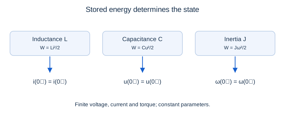
Inductance stores magnetic energy and rotor inertia stores kinetic energy. Finite power cannot change stored energy in zero time. Inductor current therefore remains continuous under finite voltage, and rotor speed under finite torque.

L is in henries, i in amperes, J in kg·m² and ω in rad/s. These energy expressions suggest the state variables. Resistance dissipates energy and adds no state of its own. Inertia is different from a pure time delay: an inertial system reacts immediately but changes gradually; a pure delay postpones the response.

The first reference: a first-order system

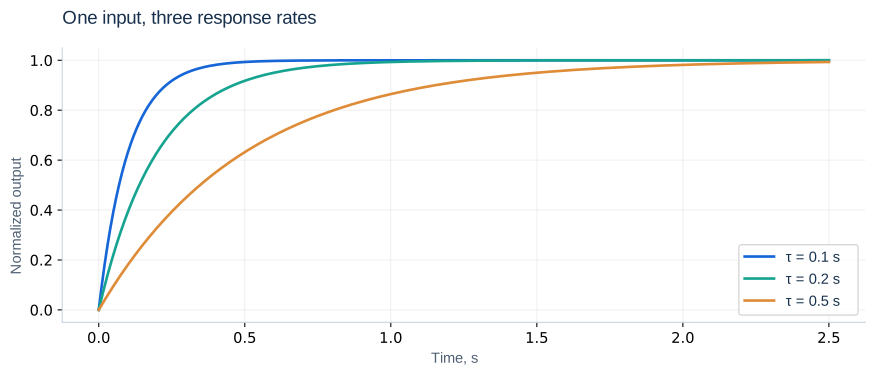
The time constant τ is measured in seconds. After τ, 36.8% of the original deviation remains; after 3τ, about 5%; after 5τ, about 0.67%. A coupled motor has two states, so its starting time is not necessarily five electrical time constants. The initial slope is (x∞ − x₀)/τ. For an exponential response, τ is the time to complete 63.2% of the total change.

Response metrics

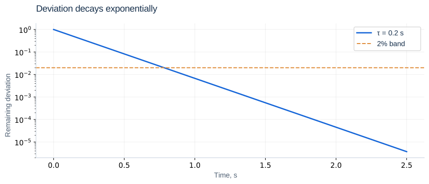
Rise time usually measures the interval from 10% to 90% of the total change. Settling time is the first time after which the response stays within a specified band around the final value. Always state that band. Overshoot measures how far the peak exceeds the final value; a monotonic exponential has none.

For a 2% band, tₛ ≈ 3.912τ: with τ = 0.2 s, this is 0.782 s. The exact exponential never reaches its final value in finite time. A practical tolerance replaces exact equality.

First calculation

import numpy as np
tau = 0.2
t = np.linspace(0, 1.2, 601)
x = 1 - np.exp(-t / tau)
settling_time = -tau * np.log(0.02)
print(f"Settling time: {settling_time:.3f} s")

Here t is an array of times and x contains the corresponding output values. This evaluates a known analytical solution; later lessons solve equations without a closed-form answer.

Switching laws and initial conditions

A state is the smallest set of quantities that, together with future inputs, determines future motion. Independent energy stores suggest inductor currents, capacitor voltages and inertial speeds. Ideal constraints may reduce the number of independent states.

With bounded voltage, i(0⁺) = i(0⁻). Similarly, capacitor voltage is continuous under bounded current, and speed under bounded torque. Their derivatives can jump. An ideal impulse violates the bounded-input assumption; its area determines the state jump. Find the old operating point, carry continuous states into 0⁺, write the new equations, and calculate the new derivatives. Do not carry old derivatives across a switch.

Forced and natural responses

For a stable linear system with a constant input, the response is a new equilibrium plus a decaying deviation. The input determines the forced component; the system dynamics and initial mismatch determine the natural component. Equilibrium need not exist: an ideal integrator with a nonzero constant input grows without limit. Check the equation before discussing a final value.

Deriving the time criteria

Normalize a nonzero change as y = (x − x₀)/(x∞ − x₀). Then y = 1 − exp(−t/τ), so the time to reach a fraction q is −τ ln(1 − q). A tolerance relative to the total change differs from one relative to the final value unless x₀ = 0. For decay to zero, use an absolute tolerance or a fraction of the initial deviation.

Example: speed rises from 20 to 80 rad/s with τ = 0.25 s. At τ it is 57.93 rad/s; rise time is 0.549 s. A 2% band of the change is ±1.2 rad/s, reached permanently after 0.978 s. Initial acceleration is 240 rad/s².

Independent exercises

1. With τ = 0.4 s, a state falls from 10 to 2. Find x(0.4) and the time to enter an absolute ±0.1 band.

2. A 0.05 H inductor carries 2 A before switching. Immediately afterwards its voltage is −10 V. Find current and its derivative at 0⁺.

Practical work

Plot responses for τ = 0.1, 0.2 and 0.5 s and calculate settling times. Repeat with x₀ = 0.4 and x∞ = 1. The initial slope changes, but τ does not. Label the normalized output and time in seconds. Explain why changing the plotted time scale does not change the physical model, and why “5τ” is only an estimate.

Calculated illustrations

Key takeaways

Inputs, stored energy and initial conditions determine a transient. Read a graph with its units and settling criterion. The exponential response is our first numerical reference.